CS777 Projectlet 3 Final Report

Nicholas Penwarden and Mohamed Eldawy

Aims

    The aim of our project was to implement a physically based simulation system. Our initial goal was to create some sort of a game where physics play a crucial role. Later we decided to shift our focus to just trying to do the simulation as fast and as accurately as possible. We experimented with several ideas to implement the same things. Our goal was to gain more understanding and insight as to the advantages and disadvantages of each method.

What we implemented

    We focused on creating spring based systems. We had a set of nodes connected with springs of varying damping and stiffness coefficients. Each node had a fixed mass. There are the internal forces of the springs, and there are external forces like gravity and wind.

In solving such a systems, we typically end up with an ordinary differential equation (ODE) describing the behavior of the system. There are several approaches to solving this ODE. In general, we have two broad classes: explicit and implicit methods.

a. Explicit methods

Explicit methods base their decision on the current state. They are not allowed to make any assumptions about the future. The simplest method is the Euler method which simply assumes the derivative is constant over an entire time step (which effectively means it uses one term of the Taylor expansion of the function). Other methods (e.g. Midpoint, Runge Kutta 4) take in to account more terms of the Taylor expansion, and therefore produce more accurate results. However, those methods require more calculations per time step.

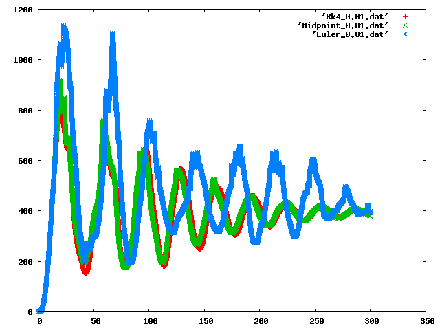
Figure 1: This graph shows the total deviation from rest length of all springs in a spring-mass system arranged in a 30x30 grid representing a piece of cloth. All methods used a constant time step of 0.01ms.

In figure 1, you can see a comparison of the various explicit methods. In that particular simulation, the only external force acting on the system is gravity. We should therefore expect the system to converge on a solution in which the internal spring forces balance with the external force of gravity. As can be seen in the graph, the extra error inherent in using the Euler method causes it to converge more slowly and less smoothly than the midpoint and RK4 methods.

The question remains as to what the time step should be in order to achieve good performance. Clearly, having finer time steps than necessary will not introduce errors in the simulation, but it may be unnecessarily costly. Having coarser time steps may cause instabilities and incorrect wrong behavior.

One of the solutions is to use adaptive time stepping. Adaptive time stepping automatically selects the appropriate time step size. This is typically done by dividing the time step in to two smaller time steps. We try taking one big step and two small steps (starting at the same point). If the error is below some threshold, the step is taken. The amount of error is then compared to the allowable error in order to determine how large the next time step should be. This method has the advantage that it will take larger steps when it is not necessary to take smaller steps.

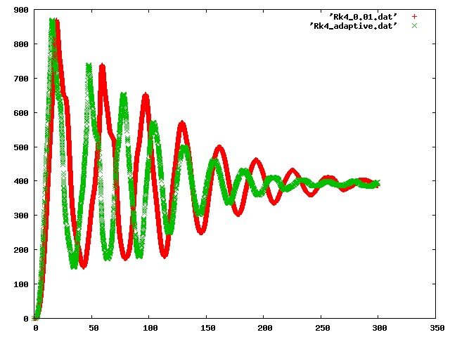
Figure 2: This graph shows the RK4 method using adaptive time stepping. Here you can see that steps are further apart during times when there is less kinetic energy in the system and closer together during times when there is more. It is interesting to note that this solution requires only 15% of the number of steps to converge as without adaptive time stepping -- and it does so more smoothly.

We implemented the Euler method, Midpoint method and Runge Kutta 4 method. We also implemented adaptive time stepping for all three.

b. Implicit method

The other way of solving the ODE is implicit solvers. Implicit solvers use the derivative at the future point for their calculation. Clearly, the derivative at the future point is still unknown (and it depends on the solution itself). This kind of dependency leads to a linear system. Solving this linear system, we obtain both the new position and derivatives of the system.

The linear system is typically sparse. The matrix of the linear system reflects the connections of the system. We used Conjugate Gradient (CG) to solve the linear system.

A naive implementation of the implicit solvers would require a 6n*6n matrix, where n is the number of nodes in the system. However, noticing that the new position can be very easily derived from the velocities, we can eliminate them from the matrix, and end up with only a 3n*3n matrix. The new matrix has half the number of elements as the original matrix. (Note that this matrix is half the size, and not one-fourth the size because of its sparsity. The other elements removed from the matrix by reducing it from 6n*6n to 3n*3n are all zero). Since the matrix is smaller, CG tends to converge faster.

We implemented the implicit method, and we implemented the optimization mentioned above to reduce the size of the system.

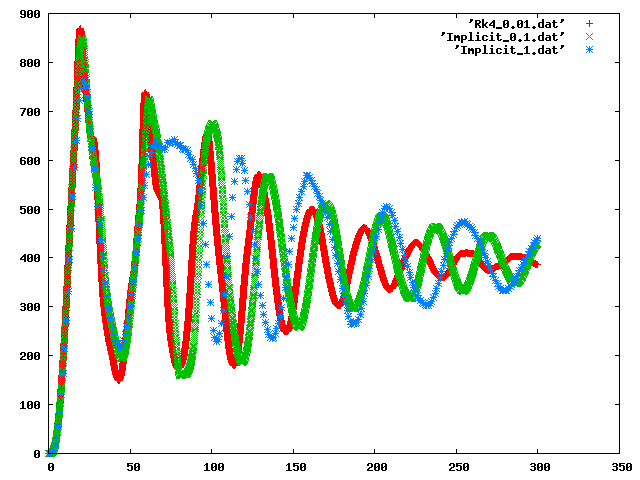
Figure 3: This image shows the implicit solver compared with the RK4 solver. Of particular interest in this graph is the fact that the implicit solver is using time steps one and two orders of magnitude larger than the RK4 solver, yet remains unconditionally stable.

c. Collision detection and handling

Being finished with the solvers themselves. We decided to focus on collision detection. We implemented collision detection and response between spring systems and some parametric surfaces (A sphere, a plane and a cube). Our collision detection was simple, we checked each node, and if it was inside the surface, a collision was reported. Handling the collision was a little trickier. Our approach to collision handling was entirely impulse based. A particle that hits a surface ends up bouncing in the reflection direction (relative to the normal vector). The new speed is equal to the original speed scaled down by the coefficient of restitution.

Our system could also handle moving obstacles. The only difference in this case is that, in collision handling, we have to calculate the relative velocities between the obstacle and the spring system. We found that especially in the case of moving obstacles, we need to have very fine steps to avoid the obstacle going through the spring system.

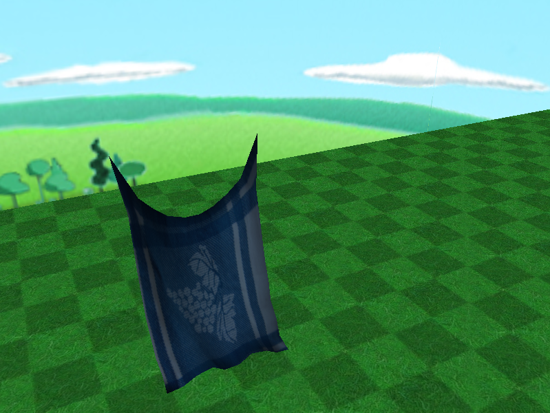
Screen shots

Here are some screen shots from our system.

1. Solving a piece of cloth using RK4

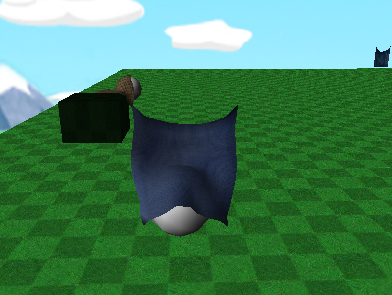
2. Doing collision detection between a piece of cloth, a sphere and a cube

3. Doing collision detection between a moving sphere and a piece of cloth

Videos

These videos are encoded using Xvid. Any standard divx decoder should be able to play them.

1. Cloth simulated with the RK4 solver
2. Cloth simulated with the RK4 solver (3 pin points)
3. Cloth falling on a sphere and cube and coming to rest
4. Cloth coming in to contact with a moving sphere

Conclusion

We successfully implemented a physically based simulator. We used both explicit and implicit methods to solve the system. The explicit method turned out to be much faster, but more susceptile to exploding. The implicit method was much slower, but provided unconditionally robust performance.

We implemented a simple collision detection and handling system. We didn't implement a self collision scheme or collision between a spring system and a mesh.