CS 777 Spring 2006 - Final Project Write-up
Davey Krill
Summary
My second and third projects were to implement a Motion Graph and be able to produce streams of motion derived from individual motion clips. This goal required solving certain sub-problems, such as identifying candidate transition points between two motion clips, selecting transition points from all the possible candidates, creating the transition motion frames between two motions, inserting them into a motion graph, and then finally pruning the graph to remove dead ends.
Once the motion graph is constructed, I should be able to generate streams of motion simply by traversing the motion graph.
Methods
The first part of this project dealt with trying to generate a simplistic motion graph data structure based on only two motion clips. I did this in order to focus most strongly on being able to detect the candidate transition points and blend motions together. Also, trying to implement a full motion graph would have been meaningless if I couldn't make it work for this base case.
Once I had this piece working, I could expand my data structure to handle an arbitrary number of motion clips.
Detecting Candidate Transition
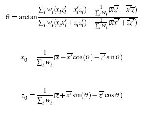
The first problem needing to be solved was to find the correct candidate transition points between two motions. This is done by finding the minimal sum of squared distances between all corresponding points in a frame pair, where one frame is from motion 1 and the second frame is from motion 2. To find the optimal 2D transformation to apply to the point cloud in motion 2, a closed-form system had to be solved.
The "distance" between frame i of the first motion and frame j of the second motion is then defined as the sum of squared distances between corresponding point clouds after the derived optimal rigid transformation is performed on the second frame point cloud:
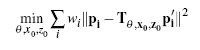
The distance is computed for every pair of frames, yielding a 2D error function for the two motions.
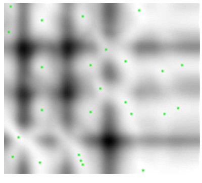
To find acceptable candidate transition points, I linearly traverse the graph looking for all local minima. This was achieved by starting at each point on the graph and walking the error function in the direction of decrease distance until it converged on a local minima. A check is performed to see if the minimal point has been added to the collection of candidate points, and if it hasn't, then it is pushed onto the stack. There are probably more efficient ways to determine the local minima points, but I found this method to work quite well.
Selecting Transition Points
Once all candidate transition points have been determined, final transition points are selected by discarding any point that falls above a determined threshold value. The choice for this threshold value was a topic for further research that did not yield any significant findings in time for submission of this project. The threshold value I used was geared towards having good transitions rather than having a highly connected graph. Typically I started with a moderately low threshold value and then tuned it even lower depending on the distance values of my candidate points.
To give an example, when dealing with the kicking motions (constrainedKicks1.bvh, constrainedKicks2.bvh, constrainedKicks3.bvh), I started with a threshold value of 60.0. This left me with approximately 20-35 points, which I could further refine to ~3-5. The threshold value for these final transition points was around 14.5. When cut frames were properly transitioned between motions, I found the results to look "good" with values as high as 30.0. My choice of a threshold value however, was more controlled by the final number of transitions I wanted between each motion clip pair rather than some static threshold value. In general, this meant the threshold value was very low.
Creating Transitions
Once a valid frame pair (i, j) has been determined, a transition is created by blending the i to i+k-1 frames of the first motion with the j-k+1 to j frames of the second motion (there was a typo in my presentation regarding which frames I was blending). k is the number of frames in the transition. First, the appropriate 2D transformation is performed on the second motion in order to align it with the first motion. Then for each frame of the transition, we linearly interpolate the root positions and perform spherical linear interpolation on joint rotations. Rp is the root position on the pth transition frame, qpi is the rotation of the ith joint on the pth frame, and a(p) is the C1-continuous blend weight.
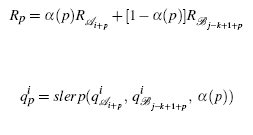
For my transitions, I used values of k=5 and k=11 in order to do a comparison between transitions with a varying number of frames. All blended sample motions included in the Results section use a value of k=11. In general, this produced the smoothest transitions.
Pruning the Graph
I took a somewhat naive approach to pruning my motion graph. Since building my motion graph, even with a small number of motion clips, took an incredibly long period of time (from what I understand, there is a much faster method for calculating distance between frames developed by Rachel that Greg and Adam used in their implementation), I searched for any nodes with very few if any outgoing edges and removed them from my graph. This allowed me to ensure that I would never hit a dead end when walking the graph, but doesn't address the issue of logical discontinuities. I was in the process of implementing the pruning algorithm discussed in the paper, but was unable to complete it.
Results
Due to the large amount of processing time necessary to construct a graph, many of my result motions are derived from only a few motion clips. However, it was not necessary to produce a very large motion graph in order the verify correctness.
To verify my distances between frames, I loaded two identical motions into my graph and outputted the error function. Predictably, it should produce a diagonal of zeros for all identically matching frames. Indeed, this was the case, as can be seen from the raw distance output here.
Once I had identified my candidate transition points, I would apply my threshold value and return only those candidate points below that value. To illustrate, here are the output files for the distances and transition points between constrainedKicks1.bvh and constrainedKicks3.bvh: distances-Kick1-3.txt, candidates-Kick1-3.txt. The list of transition points was generated with an initial threshold value of 60.0. A second selection process was applied using a threshold of 14.0 and additional selection logic was applied. For all of my examples, I gave preference to transition points that occurred in the later frames of motion one and the earlier frames of motion two. This was done to guarantee that my streams of motion made large use of both motion clips. There was no reason for me to do this other than the fact that I wanted to avoid creating motions that were predominantly one motion over the other and only used a very small piece of the second motion.
Here is a list of motions used in my motion graph: constrainedKicks1.bvh, constrainedKicks2.bvh, constrainedKicks3.bvh, constrainedFlips.bvh. All results below are generated from graph walks derived from these motions. Furthermore, I have included blended and unblended versions of each motion in order to better demonstrate the linear blending. Unfortunately, the only format I have for these motion clips are BVH, so they will require the MotionTestBedDemo project to view.
Flips-clip112-97-blended.bvh
Flips-clip112-97-unblended.bvh
The transition here occurs mid-flip and even with the linear blending there are small discontinuities due to a difference in momentum.
Kicks1-3-clip62-102-blended.bvh
Kicks1-3-clip62-102-unblended.bvh
This is one of the examples I used in my presentation to demonstrate how a low threshold value doesn't necessarily guarantee a good transition. The transition point occurs on a pair of frames that have opposing momentum. Blending does a good job of cleaning up the artifacts, but it serves as an example that there are other factors, namely momentum, that should be considered with calculating the distance between frames.
Kicks1-3-clip72-47-blended.bvh
Kicks1-3-clip72-47-unblended.bvh
Another example of how a low distance value doesn't guarantee a good transition. In this case, the transition is occurring during a period of high movement. This makes linear blending between motions tricky, especially for high values of k, since it is most likely trying to blend together poses that are very dissimilar to the actual transition point.
Kicks1-3-clip86-70-blended.bvh
Kicks1-3-clip86-70-unblended.bvh
A good motion clip with only a small artifact in the right foot.
Kicks1-3-clip90-85-blended.bvh
Kicks1-3-clip90-85-unblended.bvh
A very good motion clip with a low distance value and a good linear blend.
Kicks2-1-3-clip75-11-85-blended.bvh
This clip actually spans all three of the kicking motions. The frame pair distances are very low and linear blending does a good job of cleaning up any residual artifacts.
References
Lucas Kovar, Michael Gleicher, Frederic Pighin. Motion Graphs. ACM Siggraph 2002.